Readme File

Multi-Source Domain Adaptation for RUL Prediction of Rotating Machinery

Author: Davide Calza’
Email: davide.calza@studenti.unitn.it
:mortar_board: This project was developed in the context of the “Machine Learning for NLP II” Course of the Data Science Master’s Degree of the University of Trento

The aim of this project is to provide an exploratory analysis of Domain Adaptation (DA) techniques in the context of PHM for Bearings fault prognosis, focusing on Health Index (HI) estimation and Remaining Useful Life (RUL) prediction. The adopted dataset is the PRONOSTIA/FEMTO-ST bearings dataset.

The complete documentation can be found here.

The report can be found in the report directory.

Python version 3.11.6 was used.

Quick Start & Setup

This quick start includes steps to execute the experiments in a local settings.

Prepare the python environment: .. code-block:: bash

pip install -e .

warning:

if you want to use GPU for pytorch, follow instructions

for the setup according to your GPU and cuda version.
For the first run, be sure to set the following parameters in the config.yaml file, in order to prepare the data used by the models: .. code-block:: yaml

env:
download_dataset: true process_dataset: true extract_features: true
Edit the rest of the configuration file config.yaml and edit the parameters according to the experiment to be performed.
Run the experiment:
```
python main.py -c config.yaml -n 1
```
Results and errors can be analyzed in the errors_analysis.ipynb notebook. To visualize it, run first Jupyter Lab:
```
jupyter lab
```
and open it on the browser at localhost:8888 with the generated token. Then execute the errors_analysis.ipynb notebook.

Project Run

The file to execute to run the experiments is main.py.

python main.py -c config.yaml

information_source:

if no -c or –config flag is passed, it

will automatically use the default config.yaml file.

In order to execute multiple runs for each experiment (baseline, fine-tuning, domain adaptation: for each loss), use the -n or –nruns flag:

python main.py -c config.yaml -n <number of runs>

default is 1 run.

sos:

Example:

if we execute:
python main.py -c config.yaml -n 5
and the configuration file for the losses is the following:
weights:
  adv: 5
  daan: 0.5
  mmd: 0.3
then a total of 25 runs will be executed: 5 for the baseline, 5 for fine-tuning, 5 for adv, 5 for daan, and 5 for mmd.

It is also possible to skip baseline and fine-tuning runs by passing the flag -d or –da:

python main.py -c config.yaml -d

The reported results were produced by issuing the following command:

python main.py -c config.yaml -n 50

with the default configuration file.

Project Workflow

The entire project workflow is entirely controlled by the config.yaml configuration file (described below), and is the following:

download the dataset from the online source
convert the dataset to parquet format to speed up following steps and operations, and for achieving better compression
extract relevant features by means of DSP techniques
run the baseline model. Sources (training) experiments are filtered in order to exclude operating conditions equal to the target (test) one
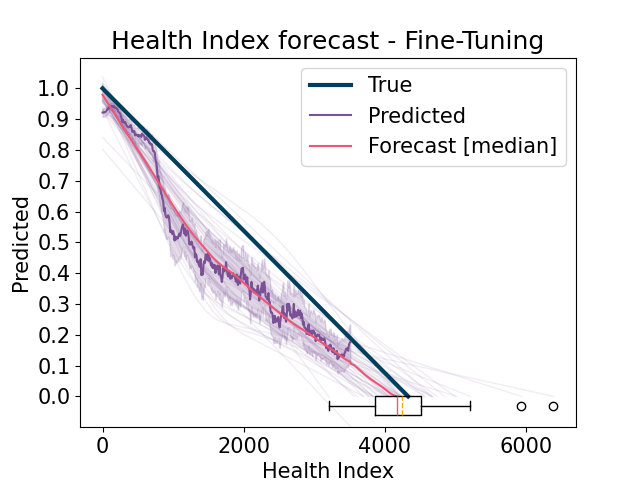
run the fine-tuning model by including sources (training) experiments that have the same operating conditions as the target (test)
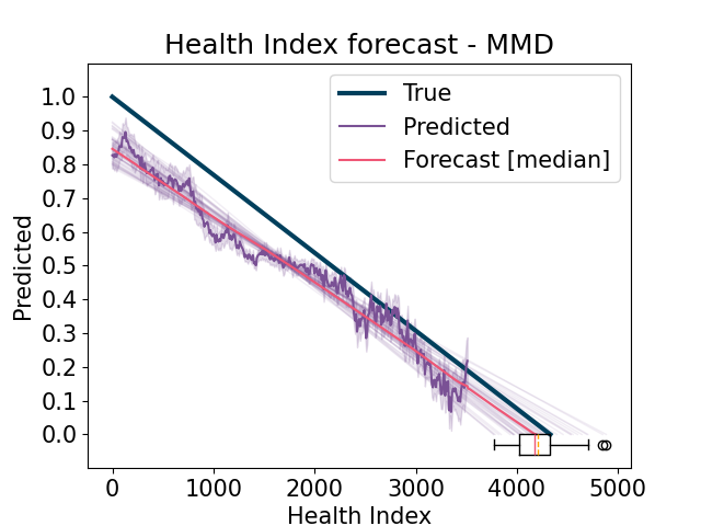
run the domain adaptation model in the same way as the fine-tuning stage, but including domain adaptation techniques

Single-Run Workflow

The workflow of the single run is the following:

Environment Setup.
Setup the execution environment by tuning pytorch parameters and setting random seeds for reproducibility. Initialize the aim run to keep track of the experiment training and results.
DataLoader Setup.
Setup the source and target datasets and their dataloaders.
Model Setup.
Training Procedure.
Train the model over the epochs and keep track of errors and metrics with aim. The number of batches per epoch is defined as the minimum of the source and target data loaders’ lengths. If the number of batches is zero, it uses the n_iter attribute of the model configuration instead. In case of a domain adaptation experiment, (i.e., da_weight > 0), the final loss is computed as the sum of the predictive network loss and the transfer loss multiplied by da_weight.
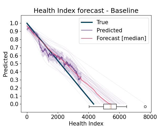
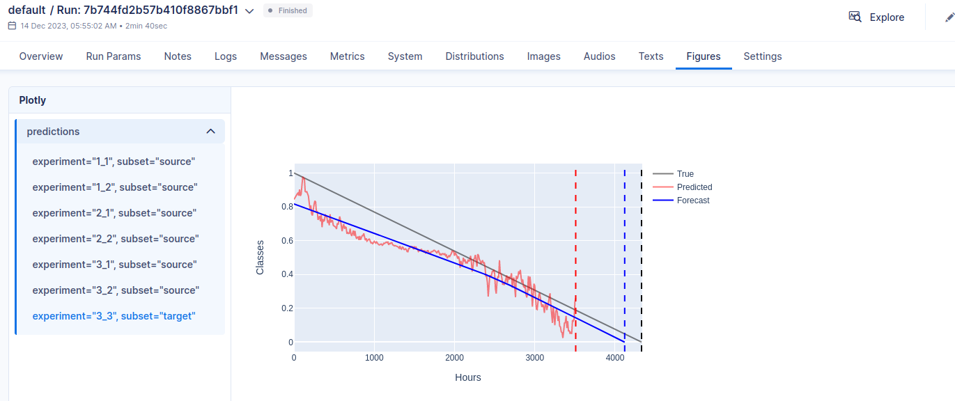
Inference Procedure.
Forecast the predicted Health Index and compute the estimated Remaining Useful Life (RUL). Compute results and errors and return visualizations. For each experiment, if it is a source (training) experiment, then use it from the Learning Set, otherwise use the complete one from the Full Test Set, in order to properly compute the scores.
Save results, weights and metadata.
Save computed results and figure and the model weights. Save also some metadata in a meta.csv file which is helpful for quickly analyzing all the performed runs and results.

Domain Adaptation

The code of the losses adopted for the domain adaptation procedure is taken and readapted from the repository DeepDA (Copyright (c) 2018 Jindong Wang licensed under MIT License) For further information please refer to the referenced repository.

warning:

different transfer losses need different transfer weights.

Refer to the weights section in the config.yaml file for their configuration. Recommended values are the ones provided with the configuration file:
weights:
  adv: 5
  daan: 0.5
  mmd: 0.3
  coral: 5e5
  bnm: 1e10

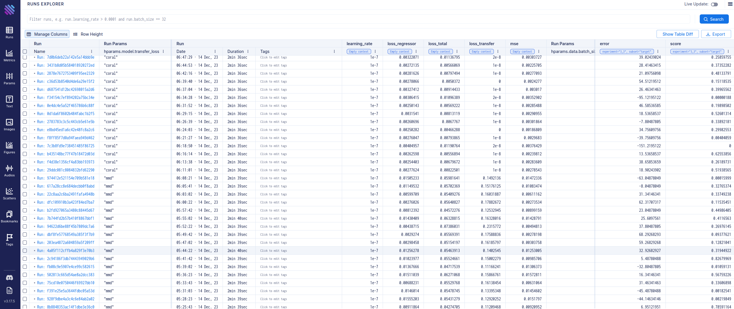
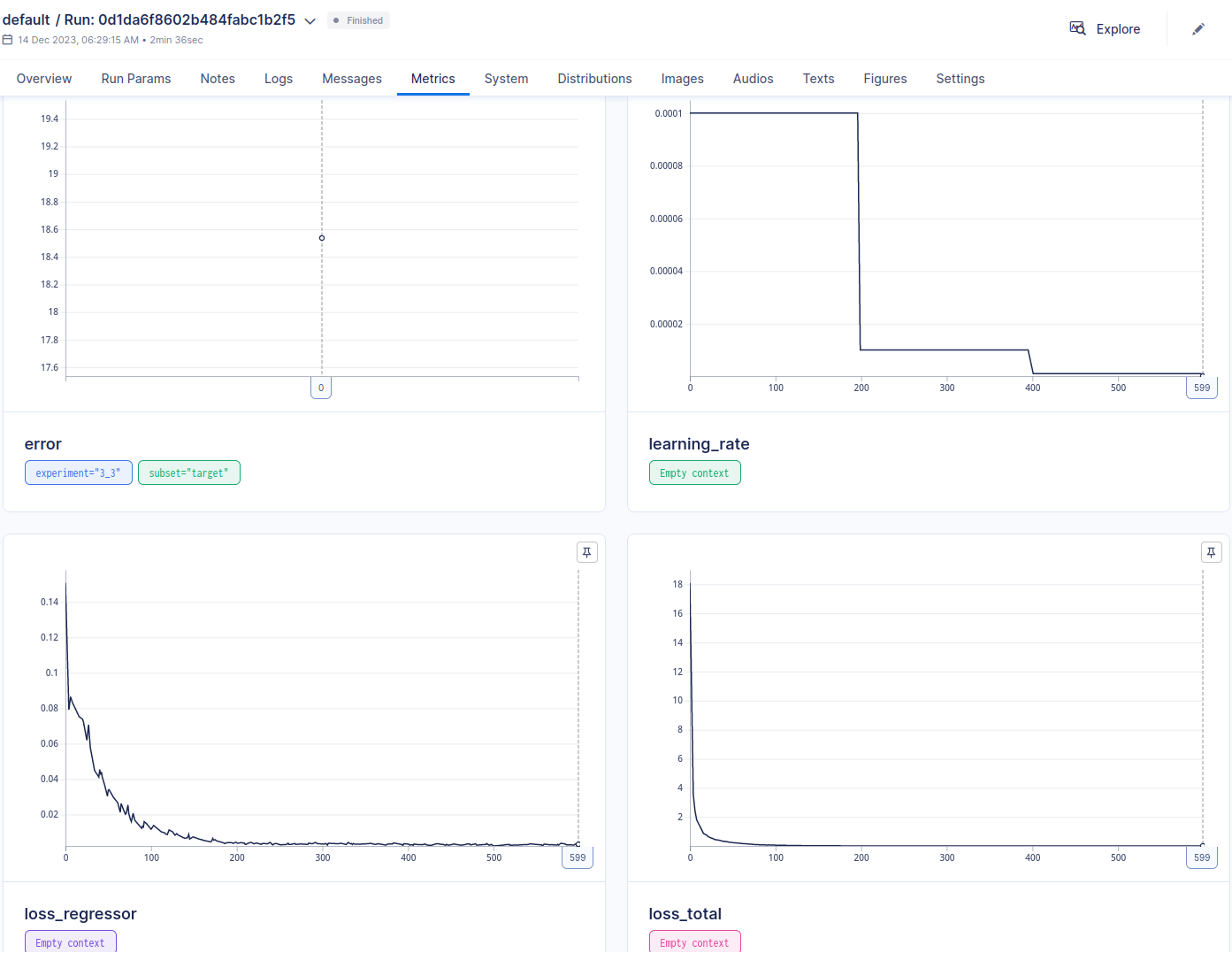
Dashboard

In order to have an overview of the ran experiments, a dashboard utility has been provided. The library used is called Aim.

To visualize the Aim dashboard, run:

aim up --repo ./data/

then open the dashboard in the browser by accessing localhost:43800.

Configuration File

The configuration file is located in the config.yaml file. The description of the parameters is as follows:

env:
  # label/name of the run
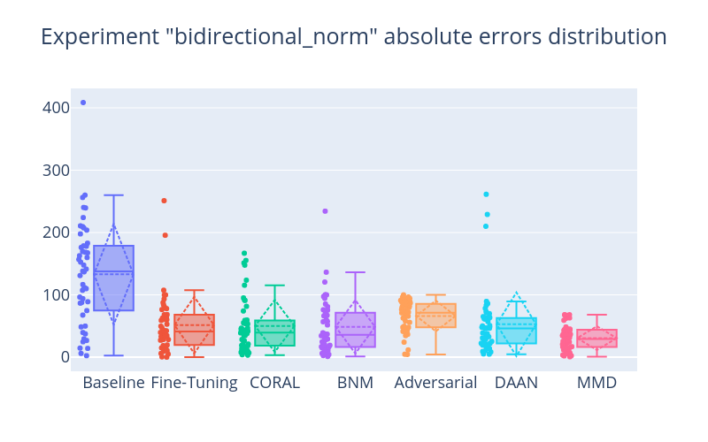
  run_name: bidirectional_norm
  # random seed. It is overridden by the seed set in the *run*
  # function
  seed: 50
  # device to run the models (cpu or cuda)
  device: cuda
  # true to download the dataset from paths.dataset
  download_dataset: true
  # true to convert raw csv to parquet files
  process_dataset: true
  # true to save parquet files with extracted MFCCs
  extract_features: true

paths:
  # url of the PRONOSTIA/FEMTO-ST dataset
  dataset: https://phm-datasets.s3.amazonaws.com/NASA/10.+FEMTO+Bearing.zip
  # directory of raw csv files
  csv: ./data/csv
  # directory of converted parquet files
  parquet: ./data/parquet
  # directory of parquet files with extracted MFCCs
  processed: ./data/processed
  # directory of the models results and weights
  output: ./data/output
  # directory of the saved scalers
  scalers: ./data/scalers
  # root directory of the aim dashboard. Final directory will be
  # <paths.aim>/.aim
  aim: ./data/

data:
  # list of experiments to use as sources. Refer to the challenge
  # description or the report for the details.
  source:
  - "1_1"
  - "1_2"
  - "2_1"
  - "2_2"
  - "3_1"
  - "3_2"
  # list of experiments to use as targets. Refer to the challenge
  # description or the report for the details.
  # Warning: multi-target experiments are not yet supported
  target:
  - "3_3"
  # list of signals to use as input for the models
  signals: ['x', 'y']
  # dataloader batch size
  batch_size: 32
  # dataset sequence length for the LSTM model
  sequence_length: 10
  # true to scale the data when loading the dataset
  scale: true

# Parameters for the MFCC feature extraction.
# Please refer to the librosa documentation for the description.
# All the parameters supported by librosa can be added.
# https://librosa.org/doc/latest/generated/librosa.feature.mfcc.html
mfcc:
  sr: 25600
  n_fft: 2560
  win_length: 2560
  hop_length: 2560
  n_mfcc: 12
  center: false
  fmin: 0.5
  fmax: 10000

model:
  # hidden dimension of the feature extraction network
  fe_hidden_dim: 128
  # output dimension of the feature extraction network
  fe_output_dim: 64
  # number of layers of the feature extraction network
  fe_num_layers: 2
  # hidden dimension of the predictive network
  hidden_dim: 128
  # transfer loss to use. Possible values are:
  # adv, daan, mmd, coral, bnm
  transfer_loss: adv
  # learning rate
  learning_rate: 0.001
  # optimizer weight decay
  weight_decay: 0.001
  # number of training epochs
  epochs: 600
  # maximum number of training iterations of the Lambda Scheduler for
  # the transfer losses
  max_iter: 600
  # network StepLR scheduler step
  scheduler_step: 200
  # network StepLR scheduler gamma
  scheduler_gamma: 0.1
  # number of training iterations per epoch if the number of batches
  # automatically computed is 0
  n_iter: 10
  # transfer weight
  da_weight: 1

# set of optimal weights for the transfer losses. They overwrite both
# model.transfer_loss and model.da_weight parameters
weights:
  adv: 5
  daan: 0.5
  mmd: 0.3
  coral: 5e5
  bnm: 1e10